WBBSE Solutions For Class 9 Maths Statistics Chapter 1 Frequency Distributions Of Grouped Data

Statistics Chapter 1 Frequency Distributions Of Grouped Data

Chapter 1 Frequency Distributions Of Grouped Data Variables or Variates

1. Suppose the weights of your classmates be x kg.
2. Then it is clear that x may take any value.
3. Because the weights of them are not equal.
4. Let the weight of one of them be 30 kg.
5. Then x = 30.
6. Again, let the weight of another of them be 32 kg.
7. Then, obviously, x = 32, i.e., x is here a changeable quantity, which is countable or measurable.
8. This x is called variable or variate.
9. Similarly, the heights of the learners of your class, and the daily expenditures of each of your families, are all variables or variates.

Definition:

Read and Learn More WBBSE Solutions For Class 9 Maths

1. The quantities, the values of which are changeable and measurable, i.e., the quantities which may take more than one value and are measurable, are called variables or variate.
2. Variables are generally of two types.

Such as—

1. Discontinuous or Discrete variables
2. Continuous variables.

1. Discontinuous or Discrete variables:

1. The variables which may take some but not all the values of a given certain limits of values are called discontinuous or discrete
2. For example, let the number of students present in a day be n.
3. Then n is a discontinuous or discrete variable.
4. Because, if the number of students in your class is 40, then the values of n may be 1,2, 3, 4,………….40; i.e, n may take only the integer values of the Certain given limit of values from 1 to 40.
5. But n is not capable to take the values of the limit like 1.5,2.5, 3.7,4.8, etc. for the number of students present on a certain day can never be an irrational one.
6. So that here n is a discontinuous or discrete variable.
7. For similar reasons, the number of students in your school, the number, of trees in your home, the population of your village, the number of calls in your mobile, etc. are all discontinuous or discrete variables.

2. Continuous variable:

1. The variables which are capable to take any value of a certain given limit and are measurable, are called continuous variables.

Such as—

Let the heights of the students in your class be x cm.

Then the values of x may be any number (rational or irrational) between 100 cm and 200 cm (if the heights of the students lie between this certain limit).

So, here x is a continuous variable.

For similar reasons, weights, temperatures, income, expenditure, etc. are all continuous variables.

This changeable but measurable characteristic of any quantity is called its numerical attributes.

Therefore, the numerical or quantitative attributes of any quantity are called variables or variates.

 

Chapter 1 Frequency Distributions Of Grouped Data  Attribute

There are some quantities that are changeable, but not measurable.

Such as the intelligence of man, merit, the educational standard of the students of class 9, the behavior of members of any family, etc.

These cannot be expressed by any quantity.

So, these qualitative quantities are called attributes.

Definition: 

The qualitative characteristics of any object or subject, which are changeable, but beyond of measurement, are called attributes.

Chapter 1 Frequency Distributions Of Grouped Data  Grouped Frequency Distribution

1. We have learned in the previous classes that by arranging the collected primary data in ascending or descending order, we get an arranged data or array.
2. These arrays when expressed in its simplest or shortest form are called frequency distribution.
3. Frequency distribution is of two types.

Such as-

1. Simple or ungrouped frequency distribution;
2. Class or grouped frequency distribution;

You have already studied a lot about the simplest or ungrouped frequency distribution. In the present chapter, we shall discuss about class or grouped frequency distribution. Before it, we shall clarify some terms regarding this.

1. Range: 

The difference between the highest and lowest values of any class or grouped data is called its range.

2. Class or Class-interval:

 If any finite grouped data be divided into some groups or classes; then each group is called its class or class interval.

In general, when the number of members of any grouped data is a large quantity, then they are grouped in such class intervals.

For example, let any grouped data of 1 to 100 be divided into 10 equal classes or class intervals as follows

1-10, 10-20, ………. 90-100.

Then, each of 1 – 10, 10 – 20, …………………….90 – 100 is a class or class interval.

3. Class frequency: 

The number of values in any class interval is called it’s class frequency.

For example, let there be 4 values of any variable of a grouped data between 1 to 10, namely 3, 5, 7, and 8.

Then, the class frequency of the class interval (110) will be 4.

4. Class limit: 

The two end values of any class interval are called the class limits of that class-intervals.

For example, the two class limits of the class intervals (110) are 1 and 10.

Class limits are of two types:

1. Lower class limit
2. Upper-class limit.

1. Lower class limit:

The class limit which is lower or smaller than the two class limits is called the lower class limit.

For example, between the two class limits 1 and 10 of the class interval (110), I am smaller than 10.

Therefore, here I am the lower class limit.

2. Upper-Class limit:

Between the two class limits of the class interval, the one which is greater is called the upper-class limit of that class interval.

Such as, in the class interval (1-10), 10 is greater than 1. 

So, here 10 is the upper class limit of the class interval (1-10).

5. Methods of formation of class intervals: 

We can form class intervals from grouped data in two methods.

Such as-

1. Exclusive method
2. Inclusive method.

1. Exclusive Method:

The method of formation of class intervals in which the upper limit of any class interval is taken as the lower limit of the next class interval and this upper limit is not included to that class interval, but is included in the next class interval is known as the exclusive method of formation of class-intervals.

For example, in the class intervals 1-10, 10-20, 20-30,……….., etc. the upper limits of each of the class intervals is the lower limit of the next class interval.

So, this is an exclusive method.

2. Inclusive Method:

The method of formation of class intervals in which both the lower and the upper limits are included to that class intervals is known inclusive method.

For example, in each of the class intervals 19, 10-19, 20-29, and 30-39,……………, both the lower and the upper limits are included in that class interval.

Hence, it is an inclusive method.

6. Class range:

The difference between the upper and the lower class limits of any class- interval is called the class range of that interval.

Such as the class range of the class interval (1-10) = (10-1) = 9 (by exclusive method) and 10 (by inclusive method).

7. Class boundary:

In order to fill up the gaps between two consecutive class intervals, the class limits of that intervals are extended to some limits, which are known as the class boundaries of that class interval.

For example, in order to fill up the gaps between 9 and 10 of the class intervals 19, 10 – 19 we can extend the intervals as follows: 0.5 9.5 and 9.5 19.5.

Thus, the class-interval 0.5 9.5, 0.5, and 9-5 are called the class boundaries.

It is clear that class boundaries are of two types-

1. Lower class boundaries.
2. Upper class- boundaries.

1. Lower Class-boundary:

The smaller one of the two class boundaries of any class interval is called the Lower class boundary.

For example, for the class interval (0.5 9.5), 0.5 is the lower class boundary.

2. Upper Class-boundary:

The greater one of the two class boundaries of any class interval is called the Upper-class boundary.

Such as, for the class interval (0.5 – 9.5), 9.5 is the upper class- boundary.

Method of finding class boundaries from class limits:

Let in the inclusive method, 10 class intervals are as follows

\(x_0-x_1, x_2-x_3, x_4-x_5, \ldots \ldots \ldots \ldots \cdot x_9-x_{10}\) and

let \(x_2-x_1=x_3-x_2=x_4-x_3=\cdots \cdots \cdots=x_9-x_8=d\) 

∴ Lower class-boundary of the class \(\left(x_0-x_1\right)=x_0-\frac{x_2-x_1}{2}=x_0-\frac{d}{2}\)

and upper class-boundary = \(x_1+\frac{x_2-x_1}{2}=x_1+\frac{d}{2}\)

Similarly, lower class-boundary of the class\(\left(x_4-x_5\right)=x_4-\frac{d}{2} \text { and upper class-boundary }=x_5+\frac{d}{2}\) 

For example, in the class intervals 1-9, 10-19, d = 10 – 9 = 1.

∴ the lower class boundary of the class \((1-9)=1-\frac{d}{2}=1-\frac{1}{2}=0.5\)

and upper class boundary = \(=9+\frac{d}{2}=9+\frac{1}{2}=9 \cdot 5\)

∴ the corresponding class will be (0.5 – 9.5).

 

8. Mid-value or class mark: The value of the variable of any class interval which lies just in the middle of the two class limits or class boundaries is called the class mark or the mid-value of that class interval.

∴ the mid-value of any class-interval = \(\frac{\text { Lower class-limit }+ \text { Upper class-limit }}{2}\)

= \(\frac{\text { Lower class-boundary }+ \text { Upper class-boundary }}{2}\)

Mathematically, if the lower-class limit or boundary of any class interval is x₁ and its upper-class limit or boundary is x₂, then

the mid-value of the class-interval = \(\frac{x_1+x_2}{2}\)

For example, the mid value of (10-12) = \(\frac{10+12}{2}\) = 11.

 

9. Class length:

The difference between the two class limits or class boundaries of any class- interval is called the class length of this class interval.

∴ Class-length = (upper class-limit) – (lower class-limit).

For example, the class length of the class interval (10 – 20) = 20 – 10 = 10

 

10. Relative frequency:

The ratio of the frequency of a certain class interval to the total frequency of any grouped data is called the relative frequency of that certain class interval.

∴ Relative frequency = \(\frac{\text { Class-frequency }}{\text { Total-frequency }}\)

For example, let the total frequency of any grouped data be 40 and that of the class-interval (10-20) be 6, then the relative frequency of (10-20) = \(\frac{6}{40}\) = 0.15.

Percentage of relative frequency:

Percentage of relative frequency = \(\frac{\text { Class-frequency }}{\text { Total-frequency }} \times 100 \%\)

 

11. Frequency density:

The ratio of the class frequency of any class interval of a grouped data to its class length is called the frequency density of that class interval.

∴ Frequency density = \(\frac{\text { Class-frequency }}{\text { Class-length }}\)

For example, if the class frequency of the class interval (10-20) is 6,

then its frequency density = \(\frac{6}{10}\)

= 0.6. [ ∵ class-length = 20- 10 = 10 ]

 

A working rule of preparation of grouped frequency distribution :

STEP-1: Express the given raw data as an array by arranging them in ascending or descending order.

STEP-2: Select the class intervals.

STEP-3: Determine the class frequency of each interval using tally marks.

STEP-4: Prepare the grouped frequency distribution table by putting class frequencies against each class interval.

 

Chapter 1 Frequency Distributions Of Grouped Data Cumulative Frequency Distribution

To know the number of values of any variable just before or next to a certain value of the variable, we generally use cumulative frequency distribution. In this table, the frequency written against any class- interval denotes the frequency of that class including the sum total of all the frequencies of the class- intervals before (or next) to that class interval.

Cumulative frequency distributions are of two types.

Such as-

1. Less than type cumulative frequency distribution
2. More than type cumulative frequency distribution.

 

1. Less than type cumulative frequency distribution :

In this type, the frequency written against any certain class interval is equal to the frequency of that class interval including the sum total of all the class intervals before that certain class interval, i.e., here. 

Cumulative frequency of the first class-interval frequency of the first class-interval.

Cumulative frequency of the second class-interval frequency of the first class-interval + frequency of the second class-interval.

Cumulative frequency of the third class-interval = frequency of the third class-interval + Cumulative frequency of the second class-interval,…………………….., etc.

For example, A distribution of the heights of 50 students of class 9 is as follows;

Table of Frequency Distribution

 

 

We can prepare a less-than-type cumulative frequency distribution table from this table as follows:

Less than type cumulative frequency distribution table

 

 

From the above table, we can say that the number of students having heights less than 160 cm = 22.

Similarly, the number of students having heights less than 170 cm = 44.

 

2. More than type cumulative frequency distribution :

In this type, the frequency written against any class interval is the frequency of that class interval including the total frequencies of its next all the class intervals, i.e., here.

Cumulative frequency of the first class interval = frequency of the first class interval + cumulative frequency of the second class interval.

Cumulative frequency of the second class interval = frequency of the second class interval + cumulative frequency of the third class interval.

Cumulative frequency of the third class interval = frequency of the third class interval + cumulative frequency of the fourth class interval.

………………………….., etc.

For example, by Preparing a more than type cumulative frequency distribution table from the above-mentioned example, we get,

More than type cumulative frequency distribution.

 

 

In the above table, the number of students having heights more than 160 cm is 28, and that more than 150 cm is 48.

 

Chapter 1 Frequency Distributions Of Grouped Data Select The Correct Answer (MCQ)

 

Question 1. Which one of the following is the pictorial representation of data?

1. Raw data
2. Bar diagram
3. Cumulative frequency
4. Frequency distribution

Solution:

2. Bar diagram is the correct

 

Question 2. The range of the data 12, 25, 15, 18, 17, 20, 22, 26, 6, 16, 11, 8, 19, 10, 30, 20, 32 is

1. 10
2. 15
3. 18
4. 26

Solution:

Given 

12, 25, 15, 18, 17, 20, 22, 26, 6, 16, 11, 8, 19, 10, 30, 20, 32.

The lowest value of the given data = 6 and the highest value = 32.

∴ the required range = 32 – 6

= 26

∴ 4. 26 is correct.

 

Question 3. The class length of 15, 610, ………………… is equal to

1. 4
2. 5
3. 4.5
4. 5.5

Solution:

The gap between (1-5) and (6-10) = d = 6 – 5 = 1

the lower-boundary of \((1-5)=1-\frac{d}{2}=1-\frac{1}{2}=0 \cdot 5\) and

∴ the upper boundary = \(5+\frac{d}{2}=5+\frac{1}{2}=5 \cdot 5\)

∴ the required class length is 5.5 – 0.5 = 5.5

∴ 2. 5.5 is correct.

 

Question 4. The mid-values of the class intervals of a frequency distribution are respectively 15, 20, 25,30, …… The class interval of which the mid-value is 20 is

1. 12.5 – 17.5
2. 17.5 – 22.5
3. 18-5 – 21.5 
4. 19.5 – 20.5 

Solution:

Given

The mid-values of the class intervals of a frequency distribution are respectively 15, 20, 25,30.

The lower class boundary of the class interval (17.5 – 22.5 ) = 17.5 and the upper class-boundary= 22.5.

∴ the mid-value of the class-interval = \(\frac{17 \cdot 5+22 \cdot 5}{2}=\frac{40}{2}=20\)

Also, its class length is 22.5 – 17.5 = 5 = (20 – 15). 

∴ 2. 17.5 – 22.5 is the correct answer.

 

Question 5. The mid-value of a class interval of a frequency distribution is 10 and the class length of each class is 6; The lower class limit of the class interval is

1. 6
2. 7
3. 8
4. 12

Solution:

Given 

The mid-value of a class interval of a frequency distribution is 10 and the class length of each class is 6.

Let the lower class limit be x. 

As per the question, the class-length of class = 6 

∴ upper class-limt = 6 + x

∴  the mid-value of the class-interval = \(\frac{x+6+x}{.2}\)

or, \(10=\frac{6+2 x}{2}\)      [∵ mid-value = 10]

or, 2x + 6 = 20

or, 2x = 20 – 6

or, 2x = 14

or, x = \(\frac{14}{2}\)

= 7.

∴ The required lower-limit = 7.

 

Chapter 1 Frequency Distributions Of Grouped Data Short Answer Type Questions

 

Question 1. Find the lower-class boundary of the continuous frequency distribution of which the mid-value is m and the upper-class boundary is u.

Solution: 

Given 

Mid-value is m and the upper-class boundary is u.

We know, mid-value of any class = \(\frac{\text { Lower class }- \text { boundary }+ \text { upper class – boundary }}{2}\)

⇒ m = \(m=\frac{\text { Lower class }- \text { boundary }+u}{2}\)

or, 2m = Lower class-boundary + u.

or, 2m – u = Lower class boundary.

∴ The required lower class-boundary=2m – u.

 

Question 2. The mid-value of a class interval of a continuous frequency distribution is 42 and its class length is 10. Find the lower and upper-class limits of the class interval.

Solution: 

Given 

The mid-value of a class interval of a continuous frequency distribution is 42 and its class length is 10.

Let the upper limit = x and lower limit = y

As per question, \(\frac{x+y}{2}\) = 42 …………….(1) and x-y = 10……………..(2);

From (1) we get, x + y = 84………………(3)

Adding (2) and (3) we get, x-y + x + y = 10 + 84

or, 2x = 94

or, x = 47.

Putting x = 47 in (2) we get, 47-y= 10

or, y = 47 – 10 

= 37.

∴ The required upper-limit= 47 and lower-limit= 37.

 

Question 3. Find the frequency density of the first class interval of the following frequency distribution :

 

 

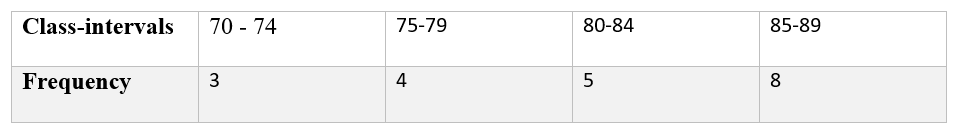
Solution:

Here, the first class interval is (70-74), the upper limit = 74, and lower-limit = 70, and d 75 – 74 = 1.

∴ upper class-boundary = 74 + \(\frac{1}{2}\) = 74.5  and lower class-boundary = 70 – \(\frac{1}{2}\) = 69.5.

∴ class-length 74.5 – 69.5 = 5.

Again, the frequency of the first class interval = 3,

∴ The required frequency density = \(\frac{\text { Class-frequency }}{\text { Class-length }}=\frac{3}{5}=0.6\)

 

Question 4. Find the relative frequency of the last class interval of question no. 3 above. 

Solution:

Here, the last class interval is (8589), the class frequency of which is 8. 

Total frequency 3+ 4+ 5+ 8 = 20

∴ the required relative frequency = \(\frac{\text { Class-frequency }}{\text { Total-frequency }}=\frac{8}{20}=0.4\)

 

Question 5. Determine which of the following are attributes and which are variables :

1. Number of members of a family 

Solution: 

The number of members of the family may be any integer, 

i.e., it may take any value.     

∴ it is a variable.

 

2. Daily temperature

Solution: 

The daily temperature may take any value.    

∴ it is a variable.

 

3. Educational standard

Solution: 

Educational standard is a non-measurable quantity.

∴  it is an attribute.

 

4. Monthly income

Solution: 

The monthly income of any person may take any value, integer, or fraction.

∴ it is a variable.

 

Chapter 1 Frequency Distributions Of Grouped Data Short Answer Type Questions

 

Question 1. The number of members of each of the 40 families in your village is given below:

 

 

 

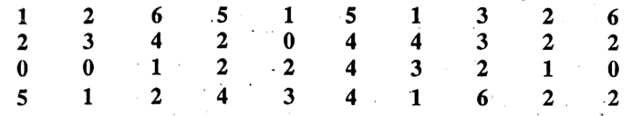
Prepare a grouped frequency distribution table of the above data taking intervals 0 – 2, 2 – 4, ………… etc.

Solution:

The given data is raw data.

Arranging them in an array, we get,

 

 

Now, using tally-mark we prepare the following grouped frequency distribution table

 

Question 2. The marks in mathematics obtained by 40 students of Hindu School, Kolkata are given below:

 

 

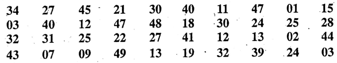
Prepare a grouped frequency distribution table of the above data taking the class intervals 1- 10, 11- 20,……………., 41 – 50.

Solution:

The lowest number obtained = 01 and the highest number obtained = 49.

in the inclusive method, we get the following table:

Grouped frequency distribution of the marks obtained in Mathematics.

 

 

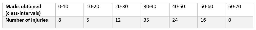
Question 3. Hindustan Times published data on the ages of some injuries of the disastrous earthquake that occurred in Nepal on 25th April 2015 as follows:

 

 

Prepare a more than type cumulative frequency distribution table of the above data. 

Solution: More than the type cumulative frequency distribution table of 300 injuries.

 

 

Question 4. Prepare a grouped frequency distribution table of the following cumulative frequency distribution:

 

 

Solution:

Here, the total number of students = 100.

In the exclusive method, the class intervals will be 0 – 10, 10-20, 20-30, 30-40, 40 – 50, 50-60, and 60-70 and the respective frequencies will be 100-92 = 8, 92-87 = 5, 87-75 = 12, 75 – 40 =35, 40 – 16 = 24, 160 = 16 and 0.

Then we get the following table